
Futures create a charting problem that stocks generally do not. An individual futures contract expires, but traders often want to view five, ten, or twenty years of uninterrupted history. Data providers solve that problem by stitching successive contracts together, and the choices they make while doing that can change the historical prices displayed on your screen.
That means two legitimate charts can tell broadly the same market story while displaying different old price levels. The sharper question inside the broader ETM lessons is therefore not simply “Which chart is right?” It is: What contracts were used, when were they switched, and was the history mathematically adjusted?
A Futures Contract Does Not Trade Forever
Start with the real exchange-listed instruments. NQZ26 is the December 2026 E-mini Nasdaq-100 futures contract; NQH27 is the March 2027 contract. They are separate contracts with their own prices, volume, open interest, and expiration dates.
When traders roll exposure, the December contract does not somehow transform into March. The trader offsets the expiring position and establishes a new position in a later contract.
The December contract does not turn into the March contract. Traders move from one contract into another.
That distinction is the foundation for everything that follows.
What a Continuous Futures Contract Actually Is
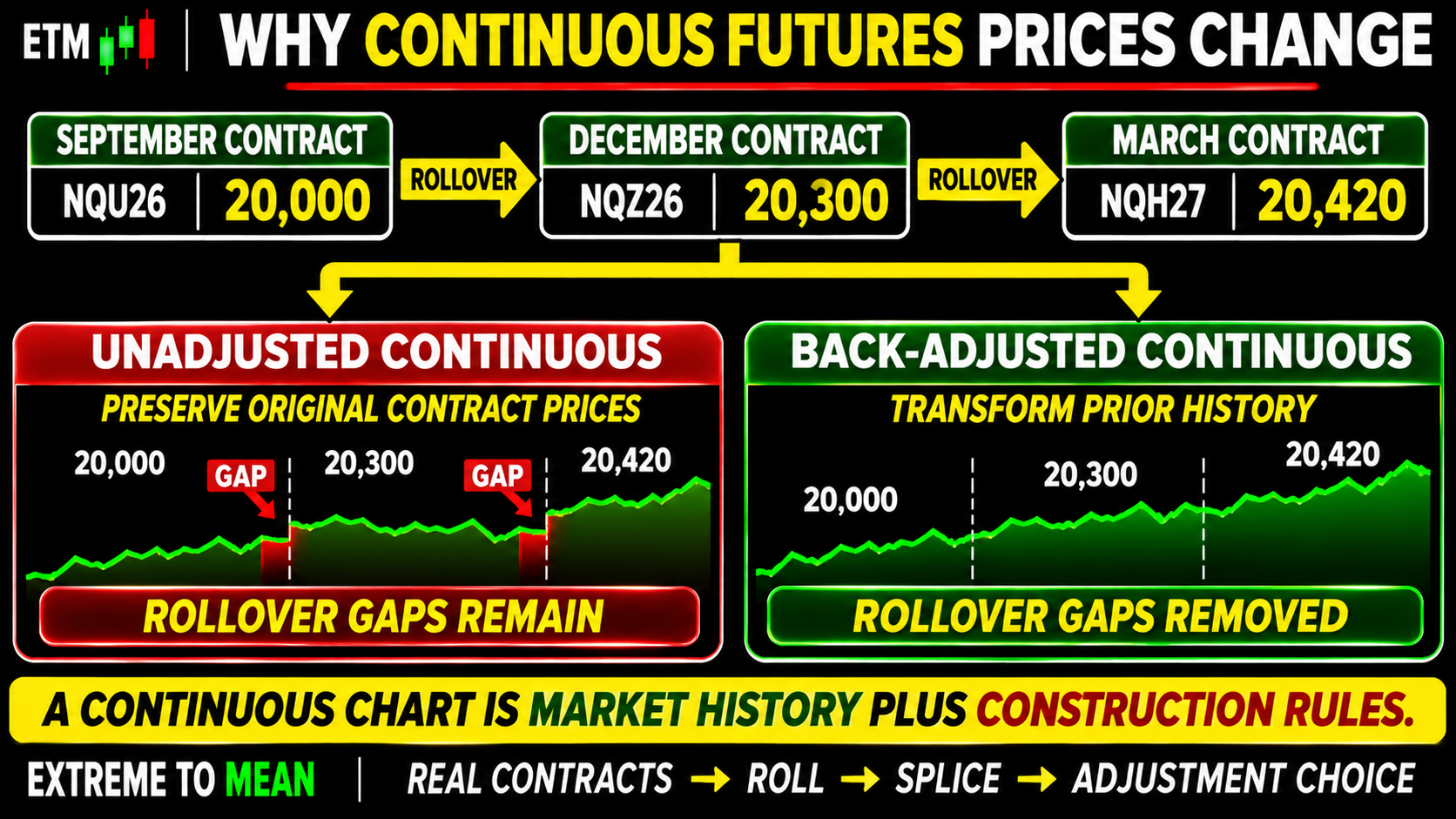
Suppose you want ten years of NQ history. Opening NQZ26 cannot give you that because the December 2026 contract exists for only a limited period. A chart provider therefore creates a continuous series by linking successive expirations into one historical chart.
A symbol such as NQ1! on TradingView is this kind of construction. It is an artificial continuous futures instrument created by linking multiple individual contract months. Historical values can therefore be synthetic rather than literal prices from one contract.
So:
ACTUAL CONTRACT ≠ CONTINUOUS SERIES.
NQ1! is useful because it gives us continuity. It is not a single CME contract that somehow traded under one identity for twenty years.
The First Hidden Choice: When Does the Chart Roll?
Before any mathematical adjustment occurs, the provider has to decide when the continuous series stops using one contract and starts using another. That decision is not universal.
CME's own continuous data distinguishes between constructions such as a liquidity-oriented Active Contract and a Front Contract based on the nearer expiration. Other providers can use their own contract-specific rollover rules, including historical volume behavior.
This explains why two platforms can disagree before either one changes a single historical price. Platform A may already be using December while Platform B is still displaying September.
Continuous futures describes a category of data series—not one universal construction method.
Why the Old and New Contracts Have Different Prices
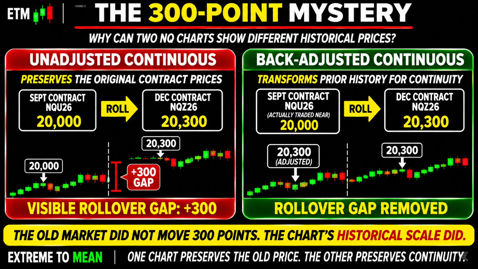
Suppose September NQ trades around 20,000 while December NQ trades around 20,300. That does not mean Nasdaq suddenly gained 300 points.
September and December are two different contracts representing exposure to different settlement dates. Differences across maturities can reflect financing, expected dividends, time to expiration, market expectations, and other term-structure effects. In commodities, storage and carry can add still more variation.
If a continuous chart stops using September at 20,000 and begins using December at 20,300, an unadjusted series can suddenly display a 300-point jump. Yet no single contract necessarily moved from 20,000 to 20,300.
A price difference between contract months is not automatically a market move.
Unadjusted Continuous Contracts: Preserve the Price, Keep the Gap
An unadjusted continuous series stitches the contracts together while preserving their original historical price values.
Using the same example:
OLD CONTRACT: 20,000
NEW CONTRACT: 20,300
The series may show:
20,000 → 20,300
The advantage is straightforward: historical contract prices remain recognizable. The disadvantage is equally important: the splice creates a discontinuity that can look like a huge market move even though the chart merely switched contracts.
Because old and new contracts generally do not trade at identical prices, simply joining them can create an artificial, non-traded return at rollover.
Raw prices can be real while the return across the splice is artificial.
Back-Adjusted Contracts: Remove the Gap, Change History
A back-adjusted continuous series takes the opposite approach. Instead of leaving the roll gap visible, the provider mathematically changes earlier historical prices so the old and new portions connect more smoothly.
Using our simplified 20,000-versus-20,300 example, earlier history might be shifted by roughly 300 points so the transition joins near 20,300.
Nothing fraudulent happened, and the provider is not claiming the old contract literally traded at that new number. The chart has transformed history for analytical continuity.
BACK-ADJUSTED PRICE ≠ LITERAL HISTORICAL TRADE PRICE.
The Market History Did Not Change—The Coordinate System Did
This is why old TradingView levels can appear to move after you enable B-ADJ or after later contract rolls alter the cumulative adjustment. Candles, swing highs, lows, price-based trendlines, and indicator inputs can all appear at different numerical values.
Suppose your old journal says you bought NQ at 19,850. Two years later, a back-adjusted continuous chart displays the same session around 20,140. Your journal did not suddenly become wrong; the continuous historical scale was transformed after subsequent rolls.
The same applies to saved screenshots. A screenshot preserves what the chart displayed at that moment, while a later back-adjusted continuous history may display a different nominal value.
The market history did not change. The coordinate system used to display that history changed.
That is why a price level only makes sense inside the coordinate system that produced it.
“Back-Adjusted” Does Not Mean One Universal Formula
There is another layer of complexity: adjustment itself is not standardized across all datasets.
Some providers use a difference-based adjustment, shifting prior history according to the old/new contract price difference near the roll. Other methodologies can use ratio adjustment, rescaling earlier prices so percentage changes are preserved more naturally.
Those approaches solve similar continuity problems differently. Difference adjustment changes historical absolute prices by adding or subtracting amounts; ratio adjustment rescales the series.
So the label back-adjusted tells you history was transformed. It does not fully tell you how.
Before arguing that one platform's 20,125 level conflicts with another platform's 20,410 level, first make sure both charts use the same roll rule and adjustment method.
Why This Matters for Indicators
Imagine an unadjusted series with an artificial 300-point roll jump. A moving average does not know the chart switched contracts; it simply sees a 300-point change.
ATR, volatility measures, momentum indicators, breakout logic, and trend calculations can react to the same discontinuity. A 200-point breakout system might even generate a signal on a 300-point rollover jump that nobody could have captured by holding one unchanged contract through the splice.
An indicator cannot know that a rollover gap was administrative unless the data tells it.
This is one reason adjusted continuous data can be valuable for longer-term trend and return analysis. A properly constructed series can remove contract-switch discontinuities that would otherwise contaminate indicators and historical signals.
Why Back-Adjusted Data Can Create Different Problems
Removing artificial roll returns solves one problem while potentially creating another.
Suppose a strategy says, “Buy NQ whenever price crosses exactly 20,000.” If earlier historical prices were repeatedly shifted by back-adjustment, some chart observations near 20,000 may represent synthetic adjusted levels that the actual contract never traded.
That matters for strategies built around absolute numbers, historical support/resistance, round-number behavior, execution prices, option strikes, spreads, or contract-specific events.
Removing fake returns can create synthetic price levels.
So a smooth chart is not automatically a valid dataset for every strategy. The dataset has to fit the question being tested.
When You Should Use the Actual Contract Instead
If your question is:
“What exact price did NQZ24 trade on September 12, 2024?”
use NQZ24.
If you are auditing an old fill, stop, entry, or execution dispute, use the actual contract involved. Never use a later back-adjusted continuous chart to conclude that an old broker fill was impossible without first checking the original contract data.
If your question is instead:
“What does the long-term trend look like across many expirations?”
a well-constructed continuous series may be much more useful.
Even when a charting platform permits trading from a continuous chart, the actual exchange order still belongs to the real underlying contract—not to an eternal synthetic continuous instrument.
A synthetic chart can generate a signal. Only an actual contract can be traded.
Continuous Contracts and Backtests
Continuous-series construction becomes especially important in research. The roll rule determines which contract supplies each historical bar, and the adjustment method determines what price history the strategy sees.
For return- and trend-based strategies, adjusted history may prevent artificial roll jumps from becoming false signals. For systems based on exact nominal prices, historical fills, contract spreads, round numbers, or expiration behavior, individual contract data may be required.
Execution modeling should also reflect what could actually have been traded. Even if a synthetic continuous series generates the signal, a realistic simulation should account for the underlying contract, rollover, tradable price, and costs.
This connects directly with what an edge actually is: a profitable historical pattern is only meaningful if the data construction represents the market question the strategy claims to exploit.
There is no universally best futures dataset. There is only a dataset fit—or unfit—for the question being tested.
The Continuous Futures Checklist
Before trusting an old futures price, indicator, or backtest, ask:
- Am I looking at a specific contract or a continuous series?
- Which real contract is currently underneath the continuous symbol?
- When does the provider switch contracts?
- Is the series adjusted or unadjusted?
- If adjusted, what method is used?
- Could later rolls have shifted my old price levels?
- Am I trying to verify an exact historical traded price?
- Could a rollover gap be creating a false indicator signal?
- Does my strategy depend on absolute price levels?
- Does my backtest model actual contract execution and rollover?
- Am I comparing two charts built with the same roll rules?
- Does this dataset actually fit the question I am asking?
These questions are part of the same discipline behind making risk clear before the trade is ready. Research inputs need the same clarity as trade inputs; otherwise we can spend hours explaining a result created by the dataset instead of the market.
The ETM Contract → Roll → Splice → Adjust → Use Framework
Use CONTRACT → ROLL → SPLICE → ADJUST → USE.
CONTRACT asks which actual expiration traded. ROLL asks when the provider moved to the next contract. SPLICE asks how successive contracts were joined, while ADJUST asks whether earlier historical prices were transformed. USE asks whether that construction is appropriate for the level, indicator, execution audit, or backtest you are performing.
The ETM free tools can support structured market research, but they cannot rescue an analysis built on misunderstood data. CHECK THE DATA BEFORE QUESTIONING THE PRICE.
Final Thought
Futures charts become confusing because contracts expire while traders want uninterrupted history. A continuous series solves that problem by stitching successive contract months together, but those contracts often trade at different prices.
An unadjusted chart preserves the historical contract values and therefore preserves roll discontinuities. A back-adjusted chart removes those discontinuities by transforming earlier history, which creates a smoother analytical series while changing the historical numbers displayed on the chart.
Neither approach is universally right or wrong. One chart may preserve the old nominal price; another may preserve analytical continuity. Different platforms can also switch contracts at different times or use different adjustment formulas and still be internally consistent.
For long-term trend work and some backtests, removing artificial roll returns can be valuable. For exact historical fills, old support levels, execution audits, or strategies built around nominal prices, the real contract may matter more.
The chart is not just market data. It is market data plus construction rules.
Educational content only. Trading involves substantial risk and is not suitable for everyone.