
Two Charts That Look Alike Are Only the Beginning
Imagine two companies operating in closely related industries. They respond to similar economic developments, and their stock prices frequently move in the same direction. When one begins outperforming the other, a trader may naturally expect the gap between them to close.
That observation can motivate a pairs-trading hypothesis, but it is not sufficient evidence for a trade. The instruments may have different price scales, sensitivities, growth prospects, or exposures, and their historical relationship may have changed for legitimate economic reasons. What looks like temporary divergence could instead be the beginning of a lasting separation.
Pairs trading generally involves establishing positions in two instruments based on expectations about their relative performance. In a common mean-reversion approach, the researcher studies whether a particular combination of their prices tends to return toward an estimated center, rather than predicting the direction of either asset independently. That shifts the question from where one asset will go to how two assets may behave relative to one another, a question that belongs in the broader Setup curriculum.
Correlation Is Not Cointegration
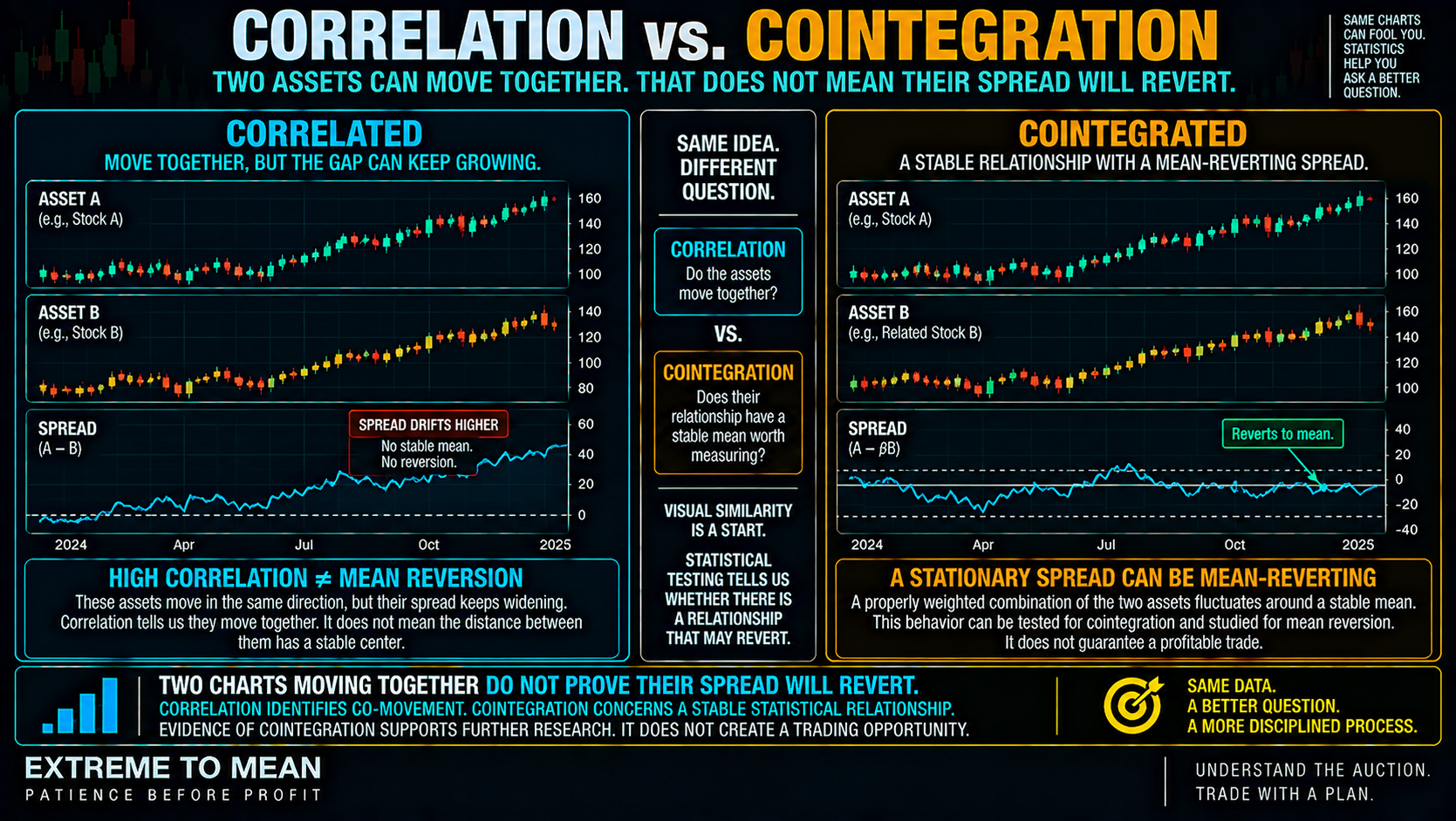
Correlation describes how two variables move together over a specified sample. Two assets can have strongly correlated daily price changes while their price levels gradually drift farther apart, leaving no stable gap for a trader to exploit. Correlation tells us that two assets have moved together; it does not prove they will return to the same relationship after moving apart.
Cointegration asks a different statistical question. Under a standard framework, suitable nonstationary price series may share a common stochastic trend such that a properly weighted combination is stationary. That constructed relationship can then be investigated for mean-reverting behavior, rather than relying on the visual similarity of the original charts.
Correlation measures co-movement over a specified sample; it does not require a stable price gap or establish reversion. Cointegration concerns a statistical long-run relationship and, under the standard framework, requires an appropriate stationary linear combination. It can justify further mean-reversion research, but it does not establish that a strategy will be profitable.
Cointegration does not require the two assets to trade at identical prices or change by equal dollar amounts. Their relationship may depend on weights estimated from historical data, and those estimates remain subject to uncertainty. Evidence of cointegration supports further investigation; it does not create a permanent promise that two prices will stay close forever.
Start With an Economic Reason, Then Challenge It
Statistical research becomes much less useful when the trader searches thousands of unrelated instruments until a handful produce attractive historical results. With enough searching, some combinations will appear unusually stable by chance, especially when the same data are repeatedly used to select and optimize the relationship. An attractive chart is not evidence that a genuine economic relationship exists.
A stronger starting point is an economically plausible connection, such as similar business exposures, related markets, or dependence on common underlying forces. That relationship motivates the research, but the data must still challenge it rather than merely confirm it. Start with a reason the relationship might exist, then use the evidence to determine whether the hypothesis deserves further investigation.
The Spread Is the Relationship We Actually Measure
In pairs trading, the spread is not necessarily the simple dollar difference between two asset prices. Researchers commonly construct a weighted combination designed to represent the relationship being studied, with a simple illustrative residual taking the form:
Sₜ = Aₜ − (α + βBₜ)
Here, Aₜ and Bₜ are the two asset prices, α is an intercept, and β is an estimated relationship coefficient. The resulting spread measures how far Asset A is from the value implied by that particular fitted relationship, rather than how many dollars separate the two quoted prices. This statistical spread is also different from the bid-ask spread that a trader pays when executing orders.
Suppose a hypothetical relationship suggests that Asset A should be approximately 10 + 0.6 × B. If Asset B trades at 100, the fitted relationship implies a value of 70 for Asset A; if Asset A instead trades at 75, the residual becomes +5. That calculation measures the deviation, but it does not establish that Asset A is overpriced or that the spread must return to zero.
The coefficient matters because different instruments may have different price scales and sensitivities to shared economic forces. Changing the weighting changes the spread and potentially the statistical relationship being examined, while the coefficient estimated in a model is not automatically an executable hedge ratio that eliminates all market risk. As the foundational mean-reversion lesson explains, defining the reference is essential before attaching trading meaning to the distance from it.
Stationarity and Testing: Does the Relationship Have a Center?
Researchers care about stationarity because it provides a statistical basis for studying fluctuations around a persistent center. In its commonly used weak form, stationarity concerns a process whose mean and covariance structure remain stable over time, rather than drifting indefinitely. A stationary spread may therefore be suitable for mean-reversion research, even when the individual asset-price series are not stationary.
One common starting assumption in the Engle–Granger framework is that the individual price series are integrated of order one, or I(1). In beginner-friendly terms, this describes a relevant class of series whose levels are nonstationary but whose first differences meet the applicable stationarity assumptions. Researchers can then estimate a relationship and use an appropriate cointegration test to examine whether the resulting residual provides evidence against the hypothesis of no cointegration.
Different statistical tests ask different questions, and they must be interpreted under their respective assumptions. An ordinary Augmented Dickey–Fuller test uses a unit-root null, while KPSS can test a null of level or trend stationarity; residual-based cointegration tests require their own appropriate procedures and critical values. No single favorable test result establishes that a relationship will remain stable indefinitely.
A mathematically defined spread is not necessarily economically meaningful. The relationship may depend on the chosen historical period, model specification, or data quality, and a finding in one sample may disappear in another. Cointegration testing helps evaluate a statistical hypothesis; it does not certify an everlasting trading relationship.
From a Defined Spread to a Z-Score
Once the spread has been constructed and its statistical properties estimated, a z-score can describe how far the current spread lies from its estimated mean in standard-deviation units. That connects directly to P058, but the earlier lesson about standardized distance remains only one part of the research. A more precise measurement of a poorly justified relationship does not make the relationship more credible.
A spread at +2.5 z may represent an unusual historical deviation, but it does not establish that convergence has begun. New information, changing liquidity, a deteriorating economic relationship, or an outdated model could explain why the spread is moving farther away. This is another application of why not every extreme is a trade: an unusual spread tells you the relationship has changed relative to its history, not whether that change is temporary.
Half-Life: How Quickly Does the Model Expect Reversion?
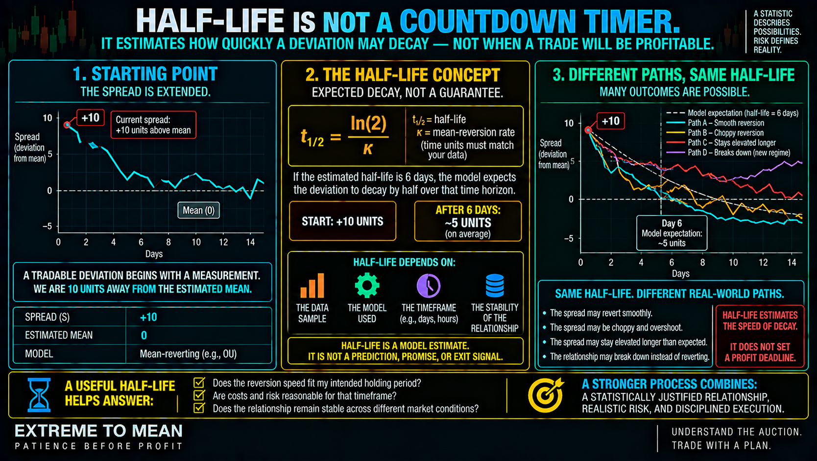
Cointegration addresses evidence about the relationship, while half-life addresses the expected speed of deviation decay under an appropriate mean-reverting model. Imagine a hypothetical model estimates a half-life of six trading days, with the current spread ten units above its estimated equilibrium. Under that model's assumptions, its conditional expected deviation would shrink to approximately five units after six trading days.
For a conventional Ornstein–Uhlenbeck model, half-life can be expressed as:
t½ = ln(2) / κ
In this formula, κ is a positive estimated mean-reversion rate expressed in consistent time units. The formula describes the time required for the model's expected deviation to decay by half, not the first time an actual spread path crosses a particular target. Half-life is a property estimated from a model, not a date on the calendar when the market owes you a profit.
The practical importance is the relationship between estimated reversion speed and the strategy's intended holding period. A trader whose process allows only short holding periods may have little use for a relationship whose estimated decay takes weeks, while a slower approach must account for capital, ongoing costs, and changing economic conditions. The estimate also depends on the model, historical sample, observation frequency, and time units, so it should never be treated as a permanent number attached to an asset pair.
The Relationship Can Break Instead of Reverting
The difficult question in pairs trading is not simply whether the spread has moved away from its historical center. It is whether the economic relationship that previously supported reversion still exists, particularly when one instrument experiences a material change that does not affect the other in the same way. Corporate restructuring, altered fundamentals, regulation, fund-composition changes, or shifting market exposures can all undermine an earlier relationship.
Temporary divergence and structural breakdown can initially look remarkably similar. In the first situation, the economic connection may remain plausible and new evidence may continue supporting the original model; in the second, the spread may establish a different center or cease exhibiting the previously observed behavior. Traders cannot reliably distinguish those outcomes from a large deviation alone, and statistical tests may not identify a structural change immediately.
That uncertainty is why a relationship needs more than a favorable historical statistic. Monitoring, predefined invalidation, position limits, and a research process that can reject the original hypothesis all matter when the spread behaves unexpectedly. The relevant question becomes whether the reason the relationship used to revert is still present, rather than how much farther the spread must travel before it finally returns.
Both Legs Have Costs, Exposures, and Execution Risk
A long-short pair is not automatically market-neutral or low-risk. The two instruments can carry different market sensitivities, volatility, liquidity, and economic exposures, and losses can occur on both legs as the relationship changes. An estimated statistical hedge ratio also has to be translated into actual positions, accounting for notional exposure, available sizes, and instrument-specific characteristics.
The theoretical spread is not an executable price by itself. A real strategy must transact in both instruments, potentially facing commissions, fees, bid-ask spreads, slippage, financing or borrow costs, and mismatched fills, while futures strategies introduce contract multipliers, expirations, and rollover considerations. The spread may revert on the chart while the costs of trading both sides consume the entire opportunity.
This is why the trade is not ready until the risk is clear. Statistical evidence may justify additional research, but it cannot substitute for understanding adverse movement, how both positions behave under stress, and what would invalidate the relationship being traded. A relationship can be statistically interesting without being economically worth trading.
Validate the Relationship Outside the Sample That Created It
Estimating a hedge ratio, testing for cointegration, selecting a spread definition, choosing parameters, and estimating half-life all introduce opportunities to fit historical noise. A pair can look exceptional when every decision has been optimized on the same dataset, then behave very differently when genuinely new observations arrive. That is why the broader distinction between a promising observation and an actual trading edge matters in this research.
The cleaner process estimates the relationship using a development period, locks the relevant methodology, and challenges it against unseen data. If the approach updates the relationship through time, the update rules must be specified in advance and use only information available at each historical decision point. Otherwise, the apparent stability may depend on future information that no live trader could have possessed.
The ETM Pairs-Trading Research Framework
The purpose of the framework is to keep relationship evidence, deviation measurement, reversion speed, and trade qualification separate. Each question should be answered before the next is allowed to support a trading conclusion, and every research finding should remain open to challenge. A useful framework must be capable of rejecting a pair even when its historical chart looks attractive.
- Economic relationship — Why might these instruments respond to common underlying forces?
- Data and horizon — What instruments, samples, observation intervals, sessions, and adjustments are being studied?
- Statistical assumptions — Are the series suitable for the proposed cointegration framework?
- Relationship and spread — What weights define the spread, and what evidence supports the estimated relationship?
- Deviation — How far is the spread from its estimated center, and how is that distance measured?
- Half-life — What model estimates the reversion speed, and what do its time units actually mean?
- Risk and tradability — Can both legs be traded with acceptable exposure, costs, execution assumptions, and defined invalidation?
- Validation — Does the relationship remain credible across different periods and genuinely unseen data?
- Decision — Should the idea be rejected, revised and retested, or advanced to further validation?
The condensed framework is Relationship → Spread → Deviation → Speed → Risk → Validation. The better question is not, “These two assets have moved apart, so how do I trade the convergence?” It is, “Do I have evidence that their constructed relationship is stable enough to investigate, and can a realistic strategy survive the time, risk, and costs involved?”
Final Thought
Pairs trading is not simply buying the asset that fell behind and shorting the asset that moved ahead. It begins with an economically plausible relationship, a carefully constructed spread, evidence that the relationship deserves mean-reversion research, and a model whose estimated decay speed makes sense for the intended horizon. Even then, the trade may not be practical or the relationship may stop behaving as it once did.
Cointegration asks whether there is evidence of a meaningful statistical relationship, the spread defines what is being measured, and half-life estimates how quickly the model expects the deviation to decay. None of those concepts independently establishes a profitable trade, and none eliminates the possibility of structural breakdown. Relationship → Spread → Deviation → Speed → Risk → Validation is the research discipline that connects the statistics to the broader Extreme to Mean system.
Educational content only. Trading involves substantial risk and is not suitable for everyone.